【CNN】深度学习专项课程学习记录10——卷积神经网络的原理和实现
时间:2023-01-21 13:30:01
学习目标
掌握卷积神经网络的原理和实现。
笔记
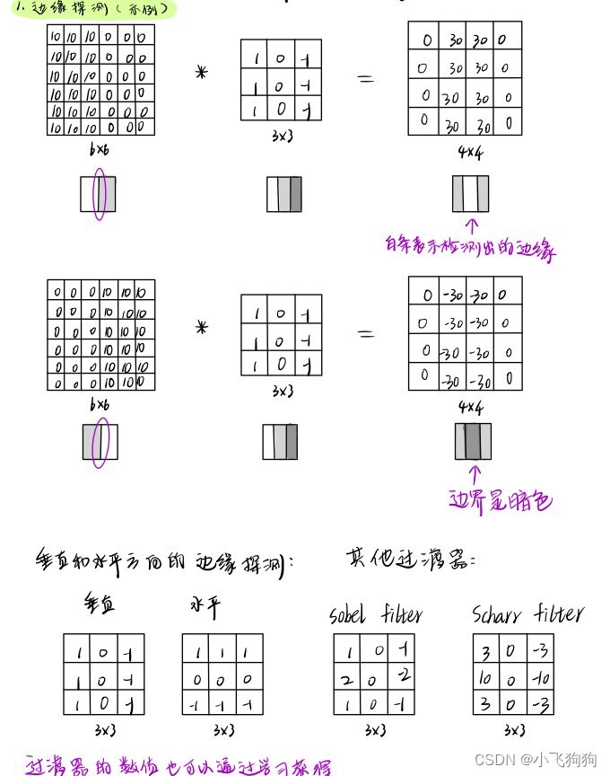
1 CNN基础知识
2 深度CNN模型:案例研究
2.1 LeNet-5(1998)
模型架构:
特点:
(1)约有6万个参数(较少);
(2)随着层数增加,通道数逐增,kernel高宽逐减;
(3)使用平均池化层;
(4)使用sigmoid/tanh(现在大部分用途Relu);
(5)池化层也采用非线性激活(现在不用)。
2.2 AlexNet
模型架构:
特点:
(1)约有6000万参数(比例)LeNet多很多);
(2)随着层数的增加,通道数逐渐增加,kernel高宽逐减;
(3)使用最大池化层;
(4)使用Relu;
(5)模型中的许多层分为两个不同的层GPU上;
(6)使用LRN层(Local Response Normalization),现在基本不用了。
2.3 VGG-16
模型架构:
特点:
(1)结构简单统一,多关注卷积层;
(2)卷积核的高宽为3x3,步长为1,padding的方式都是same;池化最大化(2)x2)池化层的步长为2;
(3)16是指该模型有16层权重;
(4)这个模型很大,共有一亿多参数;
(5)VGG-19比VGG-16更大,但性能相似,多用VGG-16。
2.4 ResNets(Residual Networks)
模型架构:
残差网络(ResNet)网络将残余块堆叠在一起。
-
残差块:
(1)原理图:
(2)当 a [ l 2 ] a^{[l 2]} a[l 2]和 a [ l ] a^{[l]} a[l]的shape同时,残差块为identity block,结构如下:
(3)当 a [ l 2 ] a^{[l 2]} a[l 2]和 a [ l ] a^{[l]} a[l]的shape不同时,残差块为convolutional block,结构如下:
-
残差网络:
特点:
(1)因为有了跳跃连接(skip connection)可以有效解决梯度消失/爆炸的问题,Resnets使得训练更深的网络成为可能。
2.5 Inception Network/GoogleNet
模型架构:
Inception网络就是将Inception模块堆叠起来的网络。
-
1x1卷积(“Network in Network”)
1x1卷积本质上是一个完全连接的神经网络,作用于 n H ∗ n W n_{H}*n_{W} nH∗nW个不同的位置;1x1卷积能够显著减少通道数 n C n_{C} nC(而池化层只能帮助减少 n H n_{H} nH和 n W n_{W} nW),从而减少计算量。 -
bottleneck
通过使用这个模块,可以显著减少参数(本例中参数数量是不用1x1卷积的情况的1/10),降低计算成本。 -
Inception模块
-
Inception网络
特点:
(1)模型结构更复杂,效果较好;
(2)不知道该怎么设置kernel的时候就用这个。
2.6 MobileNets
模型架构:
-
深度可分离卷积(Depthwise-separable convolutions):由深度卷积(Depthwise Convolution)和逐点卷积(Pointwise Convolution)两部分构成。设计这个操作的目的在于以相当低的计算成本得出具有与普通卷积中一样的输入和输出维度。
-
MobileNet v1
深度可分离卷积模块在v1网络中重复操作13次。 -
MobileNet v2
v2网络比v1网络性能更好,在于采用了Bottleneck模块。
Bottleneck在v2网络中重复操作17次。Bottleneck模块可以解决两个问题:第一,通过采用expansion操作,在模块中增加需要表现的大小,这样做可以使网络学习更丰富的功能,进行更多的计算;第二,通过采用逐点卷积/投射操作将输入值投射成较小的数值,所需存储空间减小,满足移动端使用的需求。
特点:
(1)运算成本低,占据内存较小;
(2)移动端也可以用。
2.7 EfficientNet
模型架构:
通过调整r(分辨率)、d(隐藏层的深度)、w(隐藏层的宽度)实现对模型的灵活调整。
特点:
(1)开源;
(2)使得针对特定设备自动地放大或缩小神经网络成为可能。
3 目标检测
4 迁移学习
4.1 MobileNet - v2
4.1.1 建立一个图像二分类模型
例:将在ImageNet数据集上训练好的 MobileNetv2模型,迁移到识别是否为alpaca的二分类模型。
def alpaca_model(image_shape=IMG_SIZE, data_augmentation=data_augmenter()):

    input_shape = image_shape + (3,)

    base_model = tf.keras.applications.MobileNetV2(input_shape=input_shape,
                                                   include_top=False, #重要
                                                   weights='imagenet') #imageNet

    # 冻结基准模型
    base_model.trainable = False

    # 创建输入层(输入的维度与imageNetv2相同)
    inputs = tf.keras.Input(shape=input_shape)

    # 对输入的数据进行增强
    x = data_augmentation(inputs)

    # 数据预处理
    x = preprocess_input(x)

    # 设置training为False
    x = base_model(x, training=False)

    # 使用global avg pooling
    x = tf.keras.layers.GlobalAveragePooling2D()(x)
    # 加入Dropout防止过拟合
    x = tf.keras.layers.Dropout(0.2)(x)

    # 设置只有一个神经元的输出层
    outputs = tf.keras.layers.Dense(1)(x)

    model = tf.keras.Model(inputs, outputs)

    return model
训练结果:
4.1.2 模型微调
解冻最深的层,减小学习率,以捕捉深层网络的高水平细节,尽可能提高准确率。
model2 = alpaca_model(IMG_SIZE, data_augmentation) # IMG_SIZE = (160, 160)

base_model = model2.layers[4]
base_model.trainable = True
# 打印基准模型的层数
print("Number of layers in the base model: ", len(base_model.layers))

# 从这层之后开始微调
fine_tune_at = 120

# 将 `fine_tune_at` 层之前的层都冻结起来
for layer in base_model.layers[:fine_tune_at]:
    layer.trainable = False

# 定义BinaryCrossentropy loss函数,from_logits=True
loss_function= tf.keras.losses.BinaryCrossentropy(from_logits=True)
# 定义Adam优化器,lr=0.1 * base_learning_rate
optimizer = tf.keras.optimizers.Adam(lr = 0.1 * base_learning_rate)
# 使用"accuracy"评估模型
metrics=["accuracy"]

model2.compile(loss=loss_function,
              optimizer = optimizer,
              metrics=metrics)
4.2 人脸识别(Face Recognition)和人脸验证(Face Verification)
人脸验证:“Is this the claimed person?” ——1:1匹配问题,如:检查ID card上的照片是否与真人符合;
人脸识别:“Who is this person?” ——1:K匹配问题,如:识别出屏幕前的人的身份。
4.2.1 损失函数——三元组损失(triplet loss)
triplet loss函数在训练模型的时候用到。但在搭建人脸验证和识别模型的时候,我们直接利用的是预训练的facenet,所以用不到triplet loss函数,这里说明的是triplet loss的原理。
上图表示一个锚图像(A,左),一个正例(P,中),一个反例(N,右)。triplet loss的优化方向就是使得A与P的编码距离(L2距离)最小化,A与N的编码距离(L2距离)最大化,距离之间满足(α是超参数,在此充当一个距离阈值):
∣ ∣ f ( A ( i ) ) − f ( P ( i ) ) ∣ ∣ 2 2 + α < ∣ ∣ f ( A ( i ) ) − f ( N ( i ) ) ∣ ∣ 2 2 || f\left(A^{(i)}\right)-f\left(P^{(i)}\right)||_{2}^{2}+\alpha<|| f\left(A^{(i)}\right)-f\left(N^{(i)}\right)||_{2}^{2} ∣∣f(A(i))−f(P(i))∣∣22+α<∣∣f(A(i))−f(N(i))∣∣22
整理为损失函数公式如下:
J = ∑ i = 1 m [ ∣ ∣ f ( A ( i ) ) − f ( P ( i ) ) ∣ ∣ 2 2 ⏟ (1) − ∣ ∣ f ( A ( i ) ) − f ( N ( i ) ) ∣ ∣ 2 2 ⏟ (2) + α ] + \mathcal{J} = \sum^{m}_{i=1} \large[ \small \underbrace{\mid \mid f(A^{(i)}) - f(P^{(i)}) \mid \mid_2^2}_\text{(1)} - \underbrace{\mid \mid f(A^{(i)}) - f(N^{(i)}) \mid \mid_2^2}_\text{(2)} + \alpha \large ] \small_+ J=i=1∑m[(1)
∣∣f(A(i))−f(P(i))∣∣22−(2)
∣∣f(A(i))−f(N(i))∣∣22+α]+
“ [ z ] + [z]_+ [z]+” 表示 m a x ( z , 0 ) max(z,0) max(z,0)。
注:公式里添加α的原因:在训练中增加难度,使得模型能够区分更细节的人脸差异,一般设置α=0.2。
triplet loss的代码实现如下:
def triplet_loss(y_true, y_pred, alpha = 0.2):

    anchor, positive, negative = y_pred[0], y_pred[1], y_pred[2]

    # Step 1: 计算 anchor 和 positive 的距离
    pos_dist = tf.reduce_sum(tf.square(tf.subtract(anchor,positive)),axis=-1)
    # Step 2: 计算 anchor 和 negative 的距离
    neg_dist = tf.reduce_sum(tf.square(tf.subtract(anchor,negative)),axis=-1)
    # Step 3: 计算 basic_loss
    basic_loss = tf.add(tf.subtract(pos_dist,neg_dist),alpha)
    # Step 4: 最终 loss 公式
    loss = tf.reduce_sum(tf.maximum(basic_loss,0.0))

    return loss
4.2.2 FaceNet实现人脸验证和识别
人脸验证。需要用ID card扫描机器进出的过程。
# 用 FaceNet (这里的model)形成真人照片的编码
def img_to_encoding(image_path, model):
    img = tf.keras.preprocessing.image.load_img(image_path, target_size=(160, 160))
    img = np.around(np.array(img) / 255.0, decimals=12)
    x_train = np.expand_dims(img, axis=0)
    embedding = model.predict_on_batch(x_train)
    return embedding / np.linalg.norm(embedding, ord=2)

# 验证真人是否为公司员工
def verify(image_path, identity, database, model):
    # Step 1: 首先计算摄像头拍到的真人照片的编码
    encoding = img_to_encoding(image_path,model)
    # Step 2: 计算距离:真人编码 和 ID卡上提供姓名对应的人像在公司数据库中的存照的编码
    dist = np.linalg.norm(encoding-database[identity])
    # Step 3: 如果dist < 0.7就开门
    if  dist < 0.7:
        print("It's " + str(identity) + ", welcome in!")
        door_open = True
    else:
        print("It's not " + str(identity) + ", please go away")
        door_open = False
    ### END CODE HERE
    return dist, door_open
人脸识别。不用ID card扫描,直接刷脸的过程(不需要输入员工的名字)。
def who_is_it(image_path, database, model):
    ## Step 1: 首先计算摄像头拍到的真人照片的编码
    encoding =  img_to_encoding(image_path, model)

    ## Step 2:找到数据库中编码最接近真人图像编码的员工姓名和照片编码

    # 初始化
    min_dist = 100

    # 循环遍历database的键值: names 和 encodings
    for (name, db_enc) in database.items():

        #计算L2距离
        dist = np.linalg.norm(encoding - db_enc)

        if dist < min_dist:
            min_dist = dist
            identity = name

    if min_dist > 0.7:
        print("Not in the database.")
    else:
        print ("it's " + str(identity) + ", the distance is " + str(min_dist))

    return min_dist, identity
改进人脸识别的方法:
(1)向数据库中添加更多图片;
(2)将图片去噪,裁取人脸部分。
4.3 神经风格迁移(NST, Neural Style Transfer)
文章链接: A Neural Algorithm of Artistic Style(2014)
将ImageNet上训练好的VGG-19模型,迁移到当前的任务中。
神经风格迁移要做的是将生成一张图像(G),兼具A图的内容(C)和B图的风格(S)。所以,内容损失函数 J c o n t e n t ( C , G ) J_{content}(C,G) Jcontent(C,G)在此处的作用是使得G的内容与C匹配;风格损失函数 J s t y l e ( S , G ) J_{style}(S,G) Jstyle(S,G)在此处的作用是使得G的风格与S匹配。
4.3.1 内容损失函数(Content Cost Function)
Convnet的浅层倾向于检测低水平特征,如边缘和简单的纹理;深层倾向于检测高水平特征,如复杂纹理和目标类别。The content cost takes a hidden layer activation of the neural network, and measures how different 𝑎(𝐶) and 𝑎(𝐺) are.
J c o n t e n t ( C , G ) = 1 4 × n H × n W × n C ∑ all entries ( a ( C ) − a ( G ) ) 2 J_{content}(C,G) = \frac{1}{4 \times n_H \times n_W \times n_C}\sum _{ \text{all entries}} (a^{(C)} - a^{(G)})^2 Jcontent(C,G)=4×nH<


